An Ensemble Modeling Approach for Mapping Critical Mineral

Distribution with LiDAR and PRISMA Data

Fahimeh Farahnakian

1 a

, Mahyar Youseﬁ

2 b

and Ana Cl

audia Teodoro

3 c

Geological Survey of Finland (GTK), 02151, Finland

Faculty of Engineering, Malayer University, Malayer, Iran

Instituto de Ci

encias da Terra, Departamento de Geoci

encias, Ambiente e Ordenamento do Territ

orio,

Faculdade de Ci

encias, Universidade do Porto, Porto, Portugal

ﬁ ﬁ

Keywords:

Ensemble Modeling, Data Fusion, LiDAR, PRISMA, Machine Learning, Remote Sensing, Mineral

Exploration.

Abstract:

Traditional mining exploration techniques require signiﬁcant effort, including drilling and sample collection,

making the process highly challenging and costly. The application of machine learning (ML) in mineral explo-

ration has revolutionized the ﬁeld by improving efﬁciency and accuracy in identifying critical raw materials

(CRM). This study presents a novel framework that integrates Light Detection and Ranging (LiDAR) and

PRISMA hyperspectral data with ML techniques to enhance mineral exploration. By leveraging an ensemble

model combining Random Forest (RF) and Multi-Layer Perceptron (MLP), this approach captures complex

spatial and spectral patterns, improving the prediction of cobalt, copper, and nickel concentrations. To address

the challenge of limited labeled data, synthetic samples were generated using the Gaussian Copula Synthesizer

(GCS), enhancing model generalization. The proposed methodology was validated at the

Aramo mine in As-

turias, Spain, demonstrating that the fusion of multispectral and topographical features signiﬁcantly improves

predictive accuracy. The results show that the scalability and robustness of this framework for identifying

CRM in geologically signiﬁcant yet underexplored regions.

1 INTRODUCTION

Traditional mining exploration techniques rely heav-

ily on extensive ﬁeld surveys, drilling, and geochem-

ical sampling, making the process time-consuming,

labor-intensive, and costly. Additionally, these meth-

ods often struggle with accessibility in remote or geo-

logically complex regions, limiting their efﬁciency in

large-scale mineral prospecting.

Recent advancements in Remote Sensing (RS)

technologies, particularly Light Detection and Rang-

ing (LiDAR), have been signiﬁcantly employed in

geological mapping (Paniagua et al., 1988; Putki-

nen et al., 2017) and mineral exploration (Balaram,

2023). LiDAR provides high-resolution topographi-

cal data, which makes it a valuable resource for identi-

fying the presence of minerals (Lo et al., 2021; Farah-

nakian et al., 2024a). Another useful data type for

https://orcid.org/0000-0002-7672-9346

https://orcid.org/0000-0002-8042-000X

https://orcid.org/0000-0002-8043-6431

monitoring and studying environmental phenomena

is hyperspectral data from satellites like PRISMA.

The PRISMA satellite offers high-resolution spectral

imaging across a wide range of wavelengths, allowing

for detailed analysis of surface compositions. This

capability makes it particularly useful in detecting

speciﬁc minerals and distinguishing between differ-

ent rock types or vegetation (Bedini and Chen, 2020).

Therefore, fusing these datasets provide a compre-

hensive foundation for mapping geological and min-

eralogical features (Farahnakian et al., 2024a).

Machine learning (ML) methods have been ex-

tensively applied in Mineral Prospectivity Mapping

(MPM) to analyze complex spatial and geochemical

patterns associated with mineralization. Early stud-

ies utilized traditional ML algorithms such as Sup-

port Vector Machines (SVM), which demonstrated ef-

fectiveness in binary classiﬁcation tasks for predict-

ing mineral deposits (Abedi et al., 2012). Random

Forest (RF) has gained popularity due to its robust-

ness in handling high-dimensional data and its abil-

286

Farahnakian, F., Youseﬁ, M. and Teodoro, A. C.

An Ensemble Modeling Approach for Mapping Critical Mineral Distribution with LiDAR and PRISMA Data.

DOI: 10.5220/0013493300003935

Paper published under CC license (CC BY-NC-ND 4.0)

In Proceedings of the 11th International Conference on Geographical Information Systems Theory, Applications and Management (GISTAM 2025), pages 286-296

ISBN: 978-989-758-741-2; ISSN: 2184-500X

ity to provide feature importance metrics, enabling in-

sights into the relationships between explanatory vari-

ables and mineral occurrences (Parsa and Maghsoudi,

2021). Gradient Boosting methods, such as XGBoost,

have also been employed for MPM, achieving high

accuracy by sequentially minimizing errors in predic-

tion (Ibrahim et al., 2022). Additionally, Artiﬁcial

Neural Networks (ANNs) have shown promise due

to their universal approximation capabilities, partic-

ularly in capturing complex, nonlinear relationships

between geochemical, geophysical, and RS variables

(Brown et al., 2000). Besides traditional ML models,

deep learning models such as Convolutional Neural

Networks (CNNs) (Sun et al., 2024) and autoencoders

(Luo et al., 2020) have been recently introduced to

leverage spatial and spectral features from hyperspec-

tral data, further enhancing predictive performance.

Despite these advancements, a key limitation

across most ML methods is the dependency on large,

labeled datasets for training. In mineral explo-

ration, such datasets are often limited due to the

high cost and logistical constraints of ﬁeld sam-

pling. To mitigate this issue, synthetic data genera-

tion methods, such as the Gaussian Copula Synthe-

sizer (GCS) and deep learning-based approaches like

Conditional Generative Adversarial Networks (CT-

GAN) and Tabular Variational Autoencoder (TVAE),

have been proposed to augment training datasets, en-

abling ML models to generalize better and enhance

prediction accuracy. CTGAN (Xu et al., 2019a) is

a deep learning-based model tailored for generating

synthetic tabular data, excelling at capturing complex

dependencies between features by conditioning on

discrete variables. Similarly, TVAE (Xu et al., 2019b)

leverages variational autoencoders to synthesize tabu-

lar data by effectively modeling intricate relationships

within the dataset. In this work (Farahnakian et al.,

2024a), the authors demonstrate that the GCS outper-

forms deep learning-based models such as TVAE and

CTGAN, particularly in scenarios where training data

is limited or lacks variability. Another method, SEDA

(Sheikh et al., 2024) integrates feature and distance

similarities to augment the minority samples. They

evaluated the impact of SEDA on the performance of

four ML models, including Multi-Layer Perceptron

(MLP), RF, Decision Tree (DT), and Logistic Regres-

sion (LR). Their results show that adding high-quality

synthetic samples can help ML models to generalize

better to unseen data, addressing the overﬁtting issue

commonly seen in imbalanced datasets.

This study proposes a novel approach to mineral

exploration that combines LiDAR and PRISMA hy-

perspectral data to predict concentrations of critical

minerals, including cobalt (Co), copper (Cu), and

nickel (Ni), at the

Aramo mine in Asturias, Spain.

An ensemble model combining RF and Multi-Layer

Perceptron (MLP) was developed to leverage the

strengths of both algorithms. RF was utilized for its

robust feature selection capabilities and ability to han-

dle high-dimensional datasets, while MLP was em-

ployed for its ability to model complex nonlinear re-

lationships in the fused dataset. To address the limita-

tion of labeled data, synthetic samples were generated

using GCS (Xu et al., 2019a), augmenting the dataset

and improving model performance.

The ensemble approach, employing an averaging

strategy, was evaluated using both real and synthetic

geochemical data as ground truth, demonstrating su-

perior performance compared to individual models.

Results indicate that the integration of multispectral

and topographical features derived from LiDAR and

hyperspectral imagery signiﬁcantly enhances the rep-

resentation of spatial and spectral characteristics nec-

essary for identifying mineralization zones. Addition-

ally, the results underscore the effectiveness of data

augmentation in improving ML ensemble methods

for predicting critical raw material concentrations.

This framework offers a reliable and scalable solu-

tion for mineral exploration, advancing data-driven

exploration strategies while supporting sustainable re-

source development.

2 STUDY AREA

The pilot site,

Aramo, located in the Sierra del

Aramo

in northern Spain (Figure 1), lies within the Saint

Patrick Exploration License, an area renowned for its

Co, Cu and Ni mineralization. This mineralization is

associated with the Late-Variscan

Aramo Fault (Pani-

agua et al., 1988) and occurs within the allochthonous

Aramo Unit, which is part of the Cantabrian Zone

(Aller, 1983). The mineralization predominantly oc-

curs in karstiﬁed Upper Carboniferous limestones that

have undergone multiple phases of hydrothermal al-

teration, followed by a supergene stage (

Alvarez et al.,

2018; Archibald, 2021). These distinct alteration fea-

tures, including the lithological and structural char-

acteristics of the mineralized rocks, make the Aramo

mine particularly suitable for testing and advanc-

ing RS techniques for mapping critical raw materi-

als (CRM). The diversity of alteration signatures and

the well-documented geological framework enable

researchers to calibrate and validate RS data, such as

LiDAR, hyperspectral imaging, and other methods,

for effective mineral exploration in geologically com-

plex and underexplored regions.

An Ensemble Modeling Approach for Mapping Critical Mineral Distribution with LiDAR and PRISMA Data

287

Figure 1: Location of the whole Aramo mine area. The St. Patrick mining area is the selected study area in this study.

(a) (b) (c)

Figure 2: The PRISMA imagery used in this study, alongside the actual distribution of (a) Co, (b) Cu, and (c) Ni concentrations

from geochemical data across the study area.

3 DATA

3.1 PRISMA

The PRISMA (PRecursore IperSpettrale della Mis-

sione Applicativa)

satellite provides hyperspectral

imagery across 250 bands, offering continuous spec-

tral coverage. It includes 66 bands in the Visi-

ble and Near-Infrared (VNIR) range (400–1010 nm)

and 173 bands in the Short-Wave Infrared (SWIR)

range (920–2505 nm), both with a spatial resolution

of 30 meters. Additionally, PRISMA is equipped

https://www.asi.it/en/earth-science/prisma/

with a panchromatic camera that captures a single

band (400–700 nm) image at 5-meter spatial reso-

lution. A PRISMA image of the study area, fea-

turing 5.1% cloud coverage, was acquired on May

10, 2022 (Figure 3), at the L2D processing level.

To ensure consistency, all bands were resampled us-

ing nearest-neighbor interpolation to a 5-meter reso-

lution. To reduce data dimensionality and minimize

noise, Principal Component Analysis (PCA) was em-

ployed, a technique proven effective in mineral explo-

ration with satellite imagery (Carvalho et al., 2024)

(Adiri et al., 2020). PCA compresses the information

from the original bands into a smaller set of bands,

known as principal components (PCs). Each PC rep-

S34I 2025 - Special Session on S34I - From the Sky to the Soil

288

resents contributions from all the input bands and is

ranked according to the amount of variance it explains

(Carvalho et al., 2024).

3.2 Airborne Light Detection and

Ranging (LiDAR)

In this study, high-resolution airborne LiDAR data

was acquired by Eurosense

to capture detailed topo-

graphic information of the study area. The LiDAR

survey was conducted at an altitude of approximately

2,450 meters above mean sea level (AMSL) and 1,450

meters above ground level (AGL). To ensure thorough

coverage, the LiDAR strips were ﬂown with a 70-80%

overlap, reducing gaps between ﬂight paths and en-

hancing spatial continuity.

The average LiDAR point density exceeded 10

points per square meter, providing a ﬁne spatial res-

olution, with each LiDAR spot having a ground di-

ameter of 36 cm. This high-density data was cru-

cial for producing accurate Digital Terrain Models

(DTM) and Digital Surface Models (DSM), both gen-

erated at a 0.5-meter grid resolution. This ensured

that terrain and surface details were captured with

high precision. To interpolate ground elevation values

between LiDAR points, Inverse Distance Weighting

(IDW) interpolation was applied, assigning greater

weight to points closer to the target location, thus en-

suring smooth and accurate surface modeling.

3.3 Field Data

The study area,

Aramo mine, comprises the Saint

Patrick Exploration License, for Co, Cu, and Ni,

currently being explored by AURUM Global Explo-

ration

. Figure 3 illustrates the Co deposits and their

concentration on the PRISMA image. The dataset

consists of 729 samples, with Co concentrations rang-

ing from 1 to 18,750 parts per million (ppm), with

an average of 348.9 ppm. The Cu ranges from 2 to

500,000 ppm, with an average of 10,742.7 ppm. The

Ni ranges from from 1 to 16,800 ppm, with an av-

erage of 430.7 ppm. The distribution of metal con-

centrations, particularly Cu (Cu), has a large spread,

with some extreme maximum values (e.g., 50% Cu

and 500,000 ppm Cu). The standard deviation for Cu

is quite high, indicating variability in the dataset. Co

and Ni concentrations are much lower compared to

Cu on average, and have more moderate spreads.

https://www.eurosense.com/

https://www.aurumexploration.com/

exploration-projects-in-asturias-spain/

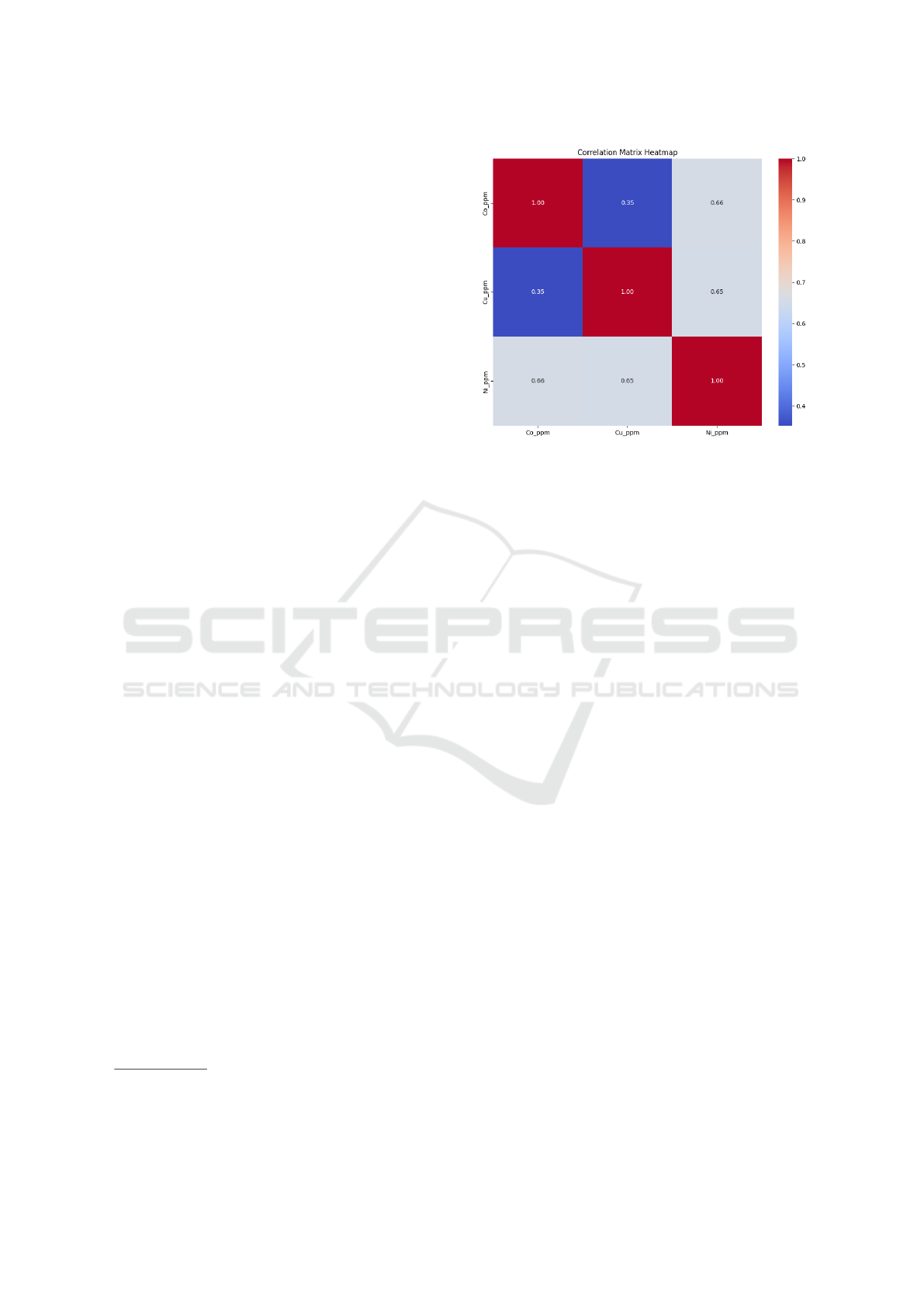
Figure 3: Correlation matrix heatmap for targets.

To conﬁrm that multi-target regression is justiﬁed,

we plot the correlation heatmaps between targets as

shown in Figure 3. From the visualization, we can

see there is a strong positive correlation between Co

and Ni (0.66). However, the correlation between Cu

and Co (0.35) is weaker. For this reason and based

on our extensive experiments, we found that using a

multi-target regression for Co and Ni and a septate

model for Cu can achieve better result based on our

data.

The original distribution of data for the three min-

erals is skewed (see Figure 4a). To address this, we

performed three preprocessing steps on the ﬁeld data

to mitigate issues such as skewed distributions, out-

liers, and variability in feature scales. The processed

distribution of minerals is presented in Figure 4b.

These preprocessing steps were crucial for enhancing

the stability and performance of the machine learning

models, as outlined below:

• Logarithmic transformation was applied to fea-

tures with positively skewed distributions to nor-

malize the data. Speciﬁcally, the natural log-

arithm with a small offset (log1p(x) = log(1 +

x)) was applied to numeric features to ensure the

transformation was deﬁned for zero values.

• Winsorization was used to handle outlier, where

feature values were capped at the 99th percentile.

This step was applied column-wise to numeric

features to reduce the effect of extreme values

while preserving the majority of the data distri-

bution.

• Standard scaling was applied to all features to

normalize their distributions. This transformation

An Ensemble Modeling Approach for Mapping Critical Mineral Distribution with LiDAR and PRISMA Data

289

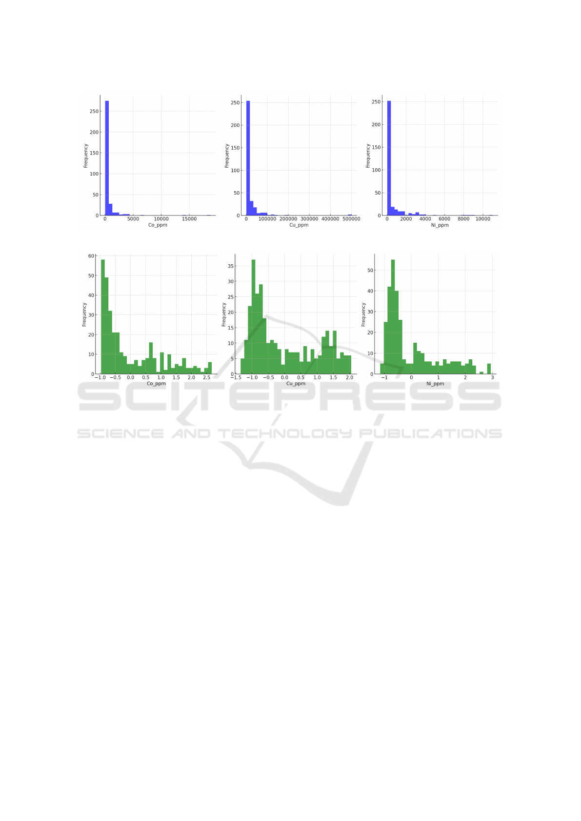
(a)

(b)

Figure 4: Comparison of (a) raw data and (b) processed distributions of mineral concentrations (Co, Cu, Ni).

scaled the data to have a mean of zero and a stan-

dard deviation of one.

4 METHODOLOGY

Figure 5 illustrates the proposed methodology out-

lined in this study. The ﬁnal dataset consists of ﬁve

features, including DEM and DSM derived from Li-

DAR data, and three principal components (PCs) ex-

tracted from PRISMA hyperspectral data. The ﬁeld

dataset, comprising 729 samples, is divided into train-

ing and test sets in a 70:30 ratio. To address the lim-

ited labeled data, GCS was employed to generate syn-

thetic data based on the training dataset. Both feature

and target values were augmented, and the synthetic

data was integrated with the original dataset to en-

hance the model training process.

Two models, RF and MLP, were used to solve the

regression problem for exploring the target mineral’s

distribution patterns. Both models are evaluated with

10-fold Cross Validation (CV), and optimal hyperpa-

rameters were determined using a Grid Search tech-

nique (Pedregosa et al., 2011). The predictions from

the two models were then combined through an av-

eraging ensemble approach to produce the ﬁnal out-

put. The ensemble model’s performance was evalu-

ated on the test dataset using metrics such as RMSE,

MAE, and R2. The best-performing model was sub-

sequently utilized to generate high-resolution mineral

prediction maps for Co, Cu, and Ni across the entire

study area.

4.1 Synthetic Data Generation

GCS is reasonable if the dataset is small, as it

helps introduce diversity while preserving relation-

ships within the data. It was ﬁrst introduced in the

Synthetic Data Vault (SDV) as a method to generate

synthetic data by modeling the statistical properties

and dependencies within a single table(Patki et al.,

2016). The process begins by identifying the appro-

priate probability distributions for each column, such

as Gaussian, uniform, or other relevant distributions,

using statistical tests like the Kolmogorov-Smirnov

(Jr., 1951) test to determine the best ﬁt. The Gaussian

Copula Synthesizer captures the covariances between

S34I 2025 - Special Session on S34I - From the Sky to the Soil

290

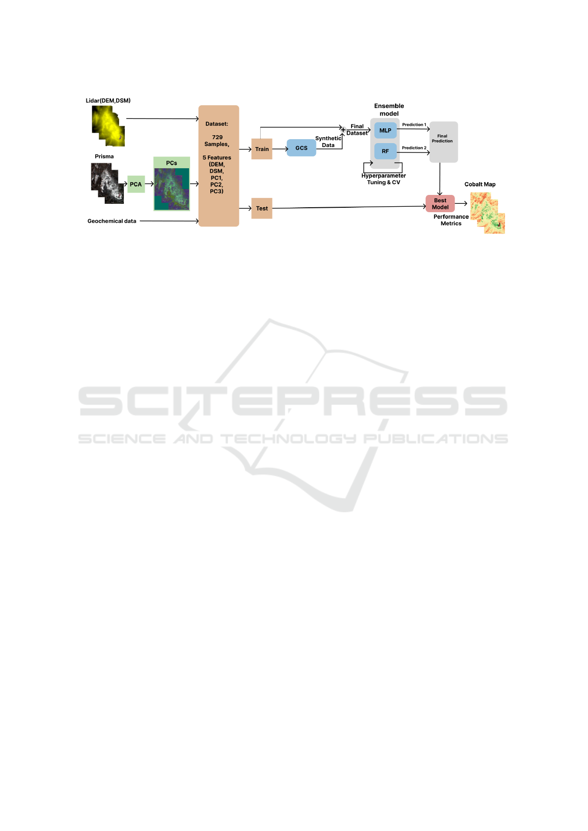
Figure 5: Overall framework.

columns by standardizing them to a normal distribu-

tion before computing their dependencies, which al-

lows it to accurately replicate the relationships within

the data. This approach ensures that the generated

data maintains the original patterns and correlations

observed in the real data, making it highly realistic

and suitable for various data science tasks.

One of the key advantages of the GCS is its com-

putational efﬁciency compared to more complex gen-

erative models, such as Generative Adversarial Net-

works (GANs). Since it relies on well-established sta-

tistical methods, this approach requires signiﬁcantly

less computational power and training time, making

it faster and more scalable for large datasets. Addi-

tionally, GCS is inherently robust and easier to imple-

ment, as it does not involve the intricate training dy-

namics of adversarial models, which can be prone to

instability and mode collapse. These strengths make

GCS an attractive choice for generating high-quality

synthetic data with minimal computational overhead,

facilitating broader adoption in scenarios where data

privacy and speed are critical concerns(Patki et al.,

2016).

4.2 Ensemble Modeling

RF (Genuer et al., 2008) is an ensemble learning al-

gorithm that constructs multiple decision trees during

training and aggregates their outputs to enhance accu-

racy and robustness. For regression tasks, RF predicts

by averaging the outputs of the individual trees, while

for classiﬁcation tasks, it determines the ﬁnal output

using the majority vote (mode) of the trees. RF excels

at handling large, high-dimensional datasets and pro-

vides inherent estimates of feature importance, offer-

ing insights into the underlying data patterns (Farah-

nakian et al., 2024b). Its design mitigates overﬁtting

by combining predictions from multiple trees, thereby

improving generalization. Recent advancements have

further reﬁned its computational efﬁciency and over-

ﬁtting control, solidifying RF as a reliable and in-

terpretable choice for both predictive and descriptive

tasks.

MLP is a type of feedforward artiﬁcial neural net-

work composed of an input layer, one or more hid-

den layers, and an output layer. Each layer consists

of interconnected neurons that employ nonlinear ac-

tivation functions to capture complex relationships in

the data. During training, MLP adjusts its weights

using optimization algorithms such as backpropaga-

tion to minimize the error between predicted and ac-

tual outputs. Known for its universal approximation

properties, MLP is highly adaptable for tasks such as

regression and classiﬁcation. However, it is suscepti-

ble to overﬁtting, especially in models with excessive

neurons or layers, which can be mitigated using tech-

niques like dropout and regularization. Determining

the optimal architecture typically requires experimen-

tation and validation.

In this study, we employed ”GridSearchCV”, a

systematic method from the scikit-learn library, to

identify the optimal set of hyperparameters for our

models. For RF, the optimal number of estimators

was 50, and the maximum depth of the trees was set

to 10. For MLP, the best conﬁguration for the hidden

layer size was 100, and the regularization term alpha

was set to 0.001.

To further enhance predictive performance, we

proposed an ensemble approach that combines the

predictions from RF and MLP to leverage their com-

plementary strengths. Ensemble learning integrates

the outputs of multiple predictive models to enhance

performance, robustness, and generalization. For re-

gression tasks, we employed an averaging-based en-

semble, which reduces variance and improves predic-

tive accuracy by merging the outputs of RF and MLP.

This approach capitalizes on RF’s ability to handle

An Ensemble Modeling Approach for Mapping Critical Mineral Distribution with LiDAR and PRISMA Data

291

noisy, high-dimensional data and MLP’s capacity to

learn from complex, multi-modal inputs, resulting in

a more robust and accurate predictive framework.

4.3 Performance Metrics

To evaluate the predictive performance of our models,

we used the following metrics:

• Mean Absolute Error (MAE): Measures the av-

erage absolute difference between predicted and

actual values. It provides a straightforward inter-

pretation of error magnitude, with smaller values

indicating better performance.

• Root Mean Squared Error (RMSE): Represents

the square root of the average squared differences

between predicted and actual values. RMSE is

sensitive to large errors and highlights the model’s

ability to handle outliers.

• Coefﬁcient of Determination (R

): Indicates the

proportion of variance in the target variable ex-

plained by the model. An R

value close to 1 sug-

gests that the model explains most of the variabil-

ity, while negative values indicate poor predictive

performance.

5 RESULTS

We trained a single-target regression model for Cu

to focus on its individual predictive patterns, while a

multi-target regression model was developed for Co

and Ni to leverage their strong correlation and en-

hance predictive performance. This dual modeling

approach ensures that both independent and corre-

lated variables are optimally modeled. The models

were evaluated using RMSE, MAE, and R², provid-

ing a comprehensive assessment of predictive accu-

racy, residual error, and the proportion of variance ex-

plained by the models.

5.1 Models’ Performance

Table 1 shows the performance of different models

(RF, MLP, and Ensemble) applied to both single-

target and multi-target regression tasks.

Single-Target Regression (Cu): The Ensemble

model demonstrated the best performance when aug-

mented data was used, achieving an RMSE of 1.66,

an MAE of 0.83, and an R² score of 0.18. This im-

provement highlights the effectiveness of GCS in en-

hancing the diversity of training data, thereby reduc-

ing model bias and variance.

RF also beneﬁted signiﬁcantly from GCS aug-

mentation, with an RMSE improvement from 2.45

(real data only) to 1.94 and a reduction in MAE from

0.92 to 0.87. However, the MLP exhibited diminished

performance with GCS augmentation, as evidenced

by an increase in RMSE (from 1.78 to 4.14) and a

slight decline in R² (from 0.11 to 0.08). This suggests

that the synthetic data may have introduced inconsis-

tencies or overﬁtting tendencies for MLP. Overall, the

Ensemble model with GCS augmentation emerged as

the most robust approach for Cu prediction, outper-

forming both individual models in accuracy and gen-

eralization.

Multi-Target Regression (Co, Ni): For the

multi-target regression of Co and Ni concentrations,

GCS augmentation provided notable beneﬁts to the

Ensemble model. The Ensemble model achieved the

best performance, with an RMSE improvement from

0.11 (real data only) to 0.10 and an increase in R² from

0.12 to 0.18. The RF model showed consistent perfor-

mance, maintaining an RMSE of 0.11 and improving

R² from 0.05 to 0.12, indicating that GCS successfully

captured additional variability in the dataset. Simi-

larly, the MLP model exhibited a slight improvement

in R² (from 0.11 to 0.14) with GCS, while maintain-

ing consistent RMSE and MAE values.

5.2 Impact of Data Augmentation on

Model Performance

Table 1 also performance metrics (RMSE, MAE,

and R²) for machine learning models trained with

and without GCS-based data augmentation for both

single-target and multi-target predictions. The col-

umn ”Data Source” in Table 1 indicates whether the

models were trained using only real data or a combi-

nation of real and synthetic data.

For the single-target predictions of Cu concentra-

tion, the RF model shows improvement with GCS

augmentation, with RMSE decreasing from 2.45 to

1.94 and R² improving from -0.67 to -0.10. However,

the MLP model’s performance slightly deteriorates

with GCS augmentation (RMSE increases from 1.78

to 4.14). The ensemble model beneﬁts from GCS aug-

mentation, achieving the best overall results for Cu

with an RMSE of 1.66 and an R² of 0.18, showcas-

ing the ensemble’s ability to generalize better when

leveraging augmented data.

For multi-target predictions (Co and Ni), the im-

pact of GCS augmentation is less pronounced but still

notable. While the RF model shows slight improve-

ments in R² from 0.05 to 0.12, the MLP and en-

S34I 2025 - Special Session on S34I - From the Sky to the Soil

292

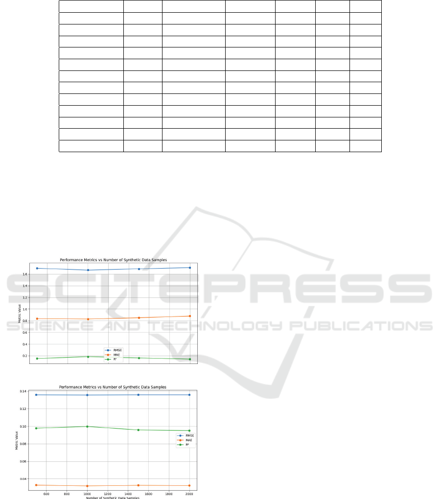
Table 1: Performance metrics for ML models with and without GCS Augmentation.

Model Type Target Data Source Model RMSE MAE R

Single-Target Cu Real Data RF 2.45 0.92 -0.67

Single-Target Cu Real + GCS RF 1.94 0.87 -0.10

Single-Target Cu Real Data MLP 1.78 0.89 0.11

Single-Target Cu Real + GCS MLP 4.14 1.15 0.08

Single-Target Cu Real Data Ensemble 1.96 0.87 -0.07

Single-Target Cu Real + GCS Ensemble 1.66 0.83 0.18

Multi-Target Co,Ni Real Data RF 0.11 0.02 0.05

Multi-Target Co,Ni Real + GCS RF 0.11 0.03 0.12

Multi-Target Co,Ni Real Data MLP 0.11 0.04 0.11

Multi-Target Co,Ni Real + GCS MLP 0.11 0.03 0.14

Multi-Target Co,Ni Real Data Ensemble 0.11 0.03 0.12

Multi-Target Co,Ni Real + GCS Ensemble 0.10 0.02 0.18

semble models beneﬁt more signiﬁcantly. The en-

semble model achieves the best overall performance

with GCS augmentation, as indicated by a decrease

in RMSE to 0.10 and an improvement in R² to 0.18.

These results suggest that GCS augmentation effec-

tively enhances model performance for multi-target

tasks, particularly for ensemble methods.

(a)

(b)

Figure 6: The performance metrics vs the number of syn-

thetic data points for the ensemble model of (a) single target

(Cu), and (b) multi-target (Co,Ni).

5.3 Model Performance vs Number of

Synthetic Samples

Different amounts of synthetic data are systematically

tested and combined with real data to enhance model

robustness. Figure 6 shows the performance metrics

(MAE, RMSE and R²) versus the number of synthetic

data points for the ensemble model of single target

and multi-target. The performance of the ensemble

model for single-target regression (Cu) improves con-

sistently as the number of synthetic data points in-

creases. As shown in Figure 6(a), the RMSE and

MAE exhibit a gradual decline, while the R² score

shows a steady increase. With the addition of up to

2,000 synthetic data samples, the RMSE reduces to

1.66, and the MAE decreases to 0.83, demonstrating

enhanced accuracy. The R² improves to 0.18, indicat-

ing better variance explanation. These results con-

ﬁrm the effectiveness of GCS augmentation in en-

hancing model robustness and predictive performance

for single-target regression tasks.

For the multi-target regression of Co and Ni, the

ensemble model similarly beneﬁts from the inclusion

of synthetic data, as shown in Figure 6(b). The RMSE

remains stable at 0.10, while the MAE maintains a

low value of 0.02. The R² score increases slightly to

0.18, demonstrating a modest improvement in vari-

ance explanation with the addition of synthetic data.

Unlike the single-target task, the improvements are

more marginal, suggesting that the real dataset al-

ready captures much of the variability for these tar-

gets. Nevertheless, the synthetic data contributes to

maintaining model stability and consistency across

performance metrics.

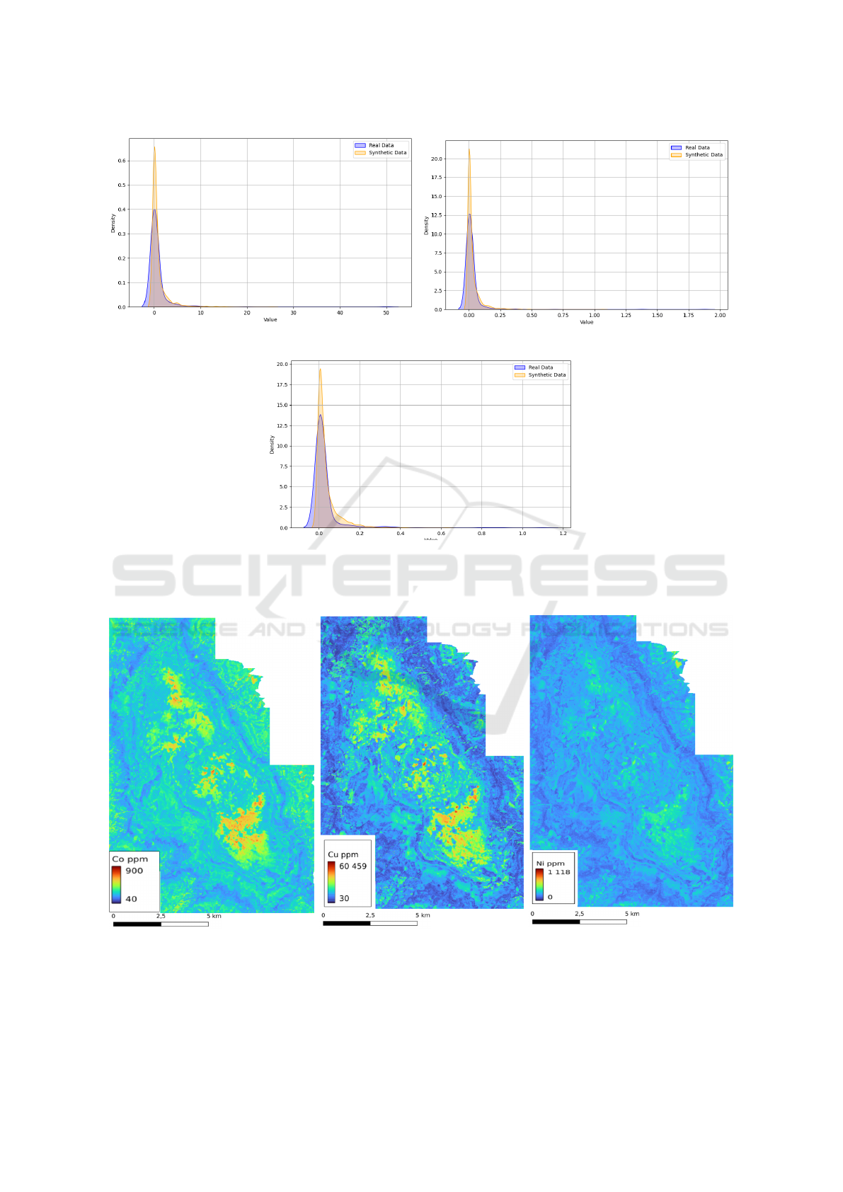
In Figure 7, we also visualize the distribution real

data and and the synthetic dataset generated using

GCS only for the optimal number of synthetic data

An Ensemble Modeling Approach for Mapping Critical Mineral Distribution with LiDAR and PRISMA Data

293

(a) (b)

(c)

Figure 7: Distribution of the real dataset versus synthetic dataset for the ensemble model predictions: (a) Cu and (b) Co and

Ni.

(a) (b) (c)

Figure 8: The prediction maps of (a) Co, (b) Cu, and (c) Ni concentrations across the study area.

S34I 2025 - Special Session on S34I - From the Sky to the Soil

294

where ensemble model achieves the lowest RMSE.

Both regression models achieve the lowest RMSE

with 2,000 synthetic samples. Across all three targets

(Cu, Co, Ni), the synthetic data closely approximates

the real data distribution. This demonstrates the ca-

pability of GCS to model and replicate the statistical

characteristics of the real dataset. The close alignment

between real and synthetic distributions supports the

validity of using the synthetic dataset for data aug-

mentation in training machine learning models. This

alignment ensures that the synthetic data does not in-

troduce signiﬁcant biases into the learning process.

5.4 Predicted Distribution Maps

The prediction maps of Co, Cu, and Ni concentrations

(Figure 8) illustrate the spatial distribution of these

critical raw materials across the study area. These

maps were generated using the ensemble modeling

approach that combines RF and MLP models using

LiDAR and PRISMA data.

The Co prediction map (Figure 8(a)) reveals a

concentrated distribution of Co in the central and

northeastern portions of the study area, with estimated

concentrations ranging from 40 ppm to 900 ppm.

These areas coincide with regions of known geologi-

cal features conducive to Co mineralization.

The Cu prediction map (Figure 8(b)) reveals a

concentrated distribution of Cu in the central and

southern portions of the study area, with estimated

concentrations ranging from 30 ppm to 60,459 ppm.

The Ni prediction map (Figure 8(c)) highlights

high Ni concentrations (up to 1,118 ppm) in the north-

ern and southern parts of the study area, indicating

potential overlap with Co mineralization zones. This

spatial correlation underscores the strong geological

relationship between Co and Ni , which was effec-

tively captured by the multi-target regression model.

These prediction maps demonstrate the efﬁcacy of

the ensemble modeling approach in integrating multi-

sensor data and leveraging synthetic data augmen-

tation to produce high-resolution distribution maps.

The results provide valuable insights for prioritizing

exploration targets and guiding resource development

strategies in geologically signiﬁcant areas.

6 CONCLUSIONS

This study presents a comprehensive framework for

mineral exploration, demonstrating the integration

of LiDAR-derived elevation models (DEM, DSM)

with hyperspectral Principal Components (PCs) ex-

tracted from PRISMA imagery provided a richer fea-

ture space for ML models. By combining the predic-

tive strengths of RF and MLP in an ensemble model,

the approach effectively addresses the complexities of

multi-sensor data analysis. The inclusion of synthetic

data generated by the GCS signiﬁcantly mitigates the

challenges posed by limited labeled datasets, enhanc-

ing model performance and generalization. Exper-

iments conducted at the

Aramo mine in Asturias,

Spain, validated the framework’s ability to produce

accurate distribution maps.

Future work will focus on extending this frame-

work to incorporate additional data sources, such as

geophysical measurements and soil geochemistry, to

further enhance prediction accuracy and applicability

in diverse geological settings. Additionally, exploring

advanced machine learning techniques, such as deep

learning models tailored for multi-sensor data fusion,

and assessing their scalability across larger study ar-

eas will be prioritized.

ACKNOWLEDGMENT

This study is funded by the European Union under

grant agreement no. 101091616, project S34I – Se-

cure and Sustainable Supply of Raw Materials for eu

Industry.

REFERENCES

Abedi, M., Norouzi, G.-H., and Bahroudi, A. (2012). Sup-

port vector machine for multi-classiﬁcation of min-

eral prospectivity areas. Computers & Geosciences,

46:272–283.

Adiri, Z., Lhissou, R., El Harti, A., Jellouli, A., and Chak-

ouri, M. (2020). Recent advances in the use of public

domain satellite imagery for mineral exploration: A

review of landsat-8 and sentinel-2 applications. Ore

Geology Reviews, 117:103332.

Aller, J. (1983). La estructura geol

ogica de la sierra del

aramo (zona cant

abrica, no de espa

na). Trabajos De

Geolog

ıa, 19(19):3–15.

Archibald, S. M. (2021). Technical report on the lrh re-

sources limited, asturmet cu-co-ni project, asturias,

nw spain. Technical report, LRH Resources Limited.

Balaram, V. (2023). Advances in analytical techniques and

applications in exploration, mining, extraction, and

metallurgical studies of rare earth elements. Miner-

als, 13(8).

Bedini, E. and Chen, J. (2020). Application of prisma satel-

lite hyperspectral imagery to mineral alteration map-

ping at cuprite, nevada, usa. Journal of Hyperspectral

Remote Sensing, 10:87.

An Ensemble Modeling Approach for Mapping Critical Mineral Distribution with LiDAR and PRISMA Data

295

Brown, W. M., Gedeon, T., Groves, D., and Barnes, R.

(2000). Artiﬁcial neural networks: a new method for

mineral prospectivity mapping. Australian journal of

earth sciences, 47(4):757–770.

Carvalho, M., Azzalini, A., Cardoso-Fernandes, J., Santos,

P., Lima, A., and Teodoro, A. (2024). Multi-sensor ap-

proach for cobalt exploration in asturias (spain) using

machine learning algorithms. In IGARSS 2024 - 2024

IEEE International Geoscience and Remote Sensing

Symposium, pages 2122–2126.

Farahnakian, F., Farahnakian, F., Sheikh, J., Downey, S.,

Williams, V., and Heikkonen, J. (2024a). Multi-modal

fusion of lidar and prisma data for cobalt mapping:

A case study from the

Aramo mine, spain. In Multi-

Modal Visual Pattern Recognition Workshop, Interna-

tional Conference on Pattern Recognition (ICPR), In-

dia. Accepted, to appear.

Farahnakian, F., Torppa, J., Luodes, N., Panttila, H., and

Karlsson, T. (2024b). A comparative study of machine

learning models for pixel-wise acid mine drainage

classiﬁcation using sentinel-2. pages 2127–2131.

Genuer, R., Poggi, J.-M., and Tuleau, C. (2008). Random

forests: some methodological insights.

Ibrahim, B., Majeed, F., Ewusi, A., and Ahenkorah, I.

(2022). Residual geochemical gold grade prediction

using extreme gradient boosting. Environmental Chal-

lenges, 6:100421.

Jr., F. J. M. (1951). The kolmogorov-smirnov test for good-

ness of ﬁt. Journal of the American Statistical Associ-

ation, 46(253):68–78.

Lo, P.-C., Lo, W., Wang, T.-T., and Hsieh, Y.-C. (2021). Ap-

plication of geological mapping using airborne-based

lidar dem to tunnel engineering: Example of don-

gao tunnel in northeastern taiwan. Applied Sciences,

11:4404.

Luo, Z., Xiong, Y., and Zuo, R. (2020). Recognition of geo-

chemical anomalies using a deep variational autoen-

coder network. Applied Geochemistry, 122:104710.

Paniagua, A., Loredo, J., and Garcia Iglesias, J. (1988). Ep-

ithermal (cu-co-ni) mineralization in the aramo mine

(cantabrian mountains, spain): Correlation between

paragenetic and ﬂuid inclusion data. Bulletin de

Min

eralogie, 111(3):383–391.

Parsa, M. and Maghsoudi, A. (2021). Assessing the effects

of mineral systems-derived exploration targeting cri-

teria for random forests-based predictive mapping of

mineral prospectivity in ahar-arasbaran area, iran. Ore

Geology Reviews, 138:104399.

Patki, N., Wedge, R., and Veeramachaneni, K. (2016).

The synthetic data vault. In 2016 IEEE International

Conference on Data Science and Advanced Analytics

(DSAA), pages 399–410.

Pedregosa, F., Varoquaux, G., Gramfort, A., Michel, V.,

Thirion, B., Grisel, O., Blondel, M., Prettenhofer,

P., Weiss, R., Dubourg, V., Vanderplas, J., Passos,

A., Cournapeau, D., Brucher, M., Perrot, M., and

Duchesnay,

E. (2011). Scikit-learn: Machine learn-

ing in python. Journal of Machine Learning Research,

12:2825–2830.

Putkinen, N., Eyles, N., Putkinen, S., Ojala, A., Palmu,

J.-P., Sarala, P., V

anen, T., R

ais

anen, J., Saare-

lainen, J., Ahtonen, N., R

onty, H., Kiiskinen, A.,

Rauhaniemi, T., and Tervo, T. (2017). High-resolution

lidar mapping of glacial landforms and ice stream

lobes in ﬁnland. Bulletin of the Geological Society

of Finland, 89.

Sheikh, J., Farahnakian, F., Farahnakian, F., Zelioli, L., and

Heikkonen, J. (2024). SEDA: Similarity-Enhanced

Data Augmentation for Imbalanced Learning, pages

32–47.

Sun, K., Yansi, C., Geng, G., Lu, Z., Zhang, W., Song, Z.,

Guan, J., Zhao, Y., and Zhang, Z. (2024). A review

of mineral prospectivity mapping using deep learning.

Minerals, 14:1021.

Xu, L., Skoularidou, M., Cuesta-Infante, A., and Veera-

machaneni, K. (2019a). Modeling tabular data using

conditional gan. Advances in neural information pro-

cessing systems, 32.

Xu, L., Skoularidou, M., Cuesta-Infante, A., and Veera-

machaneni, K. (2019b). Modeling tabular data using

conditional gan. Advances in Neural Information Pro-

cessing Systems (NeurIPS).

Alvarez, R., Ord

nez, A., P

erez, A., De Miguel, E., and

Charlesworth, S. (2018). Mineralogical and environ-

mental features of the asturian copper mining district

(spain): A review. Engineering Geology, 243:206–

217.

S34I 2025 - Special Session on S34I - From the Sky to the Soil

296